0%

SCS in LINC PA

LINC (Linear amplification with nonlinear components) 是一种使用非线性元件进行线性放大的功率放大器系统,可以在获得高线性度的同时获得高效率。其结构如下图所示:

LINC

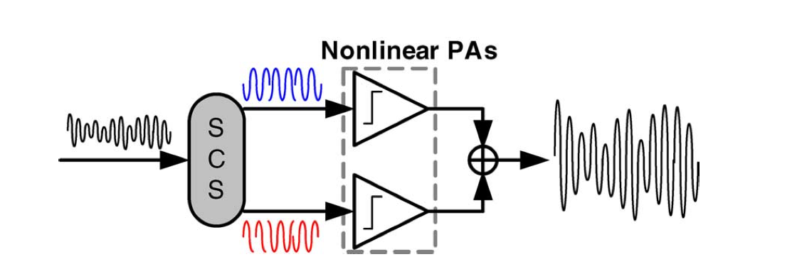
LINC 的基本思想是使用 SCS (signal component separator) 将相位幅度调制的信号转为两路相位调制信号,然后再通过两个高效率的非线性功率放大器放大,最后通过组合两路信号获得原始信号的放大后的信号。

在 LINC 系统中,需要使用到 SCS,其实现可以使用模拟的方案,也可以使用全数字的方案。

本文记录了全数字 SCS 的实现方法。

基于 CORDIC 算法的 SCS 原理

image-20210411155141497

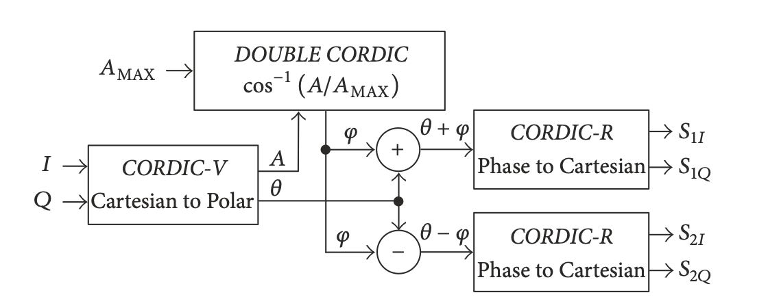
基于 CORDIC 算法的 SCS 原理图如上图所示,基带信号 I Q 经过 CORDIC-V 模块,从笛卡尔转换到极坐标,得到振幅 \(A\) 和相位 \(\theta\),振幅 \(A\) 经过 DOUBLE CORDIC 模块,进行 \(\rm{cos}^{-1}(A/A_{MAX})\) 的运算,得到 \(\varphi\),相当于把振幅信号转为相位信号。然后通过两个 CORDIC-R 模块,分别对 \(\theta + \varphi\)\(\theta - \varphi\) 做相位到笛卡尔坐标的转换,得到四路调相信号:\(S_{1I},S_{1Q},S_{2I},S_{2Q}\)

具体计算过程如下:

假设基带信号 (baseband signal) 为: \[ S_b(t)=S_i(t)+jS_q(t) \] 则频带信号 (transmitted signal) 可以表示为: \[ S(t)=Re\left\{ (S_i(t)+jS_q(t))e^{j\omega _ct} \right\}=A(t)\cos\left(w_{c}t+\theta(t)\right) \] DOUBLE CORDIC\[ \phi(t)=\cos^{-1}\left(A(t)/A_{\max}\right) \] CORDIC-R\[ S_{1I}(t) = 0.5 A_{max} \rm{cos}[\theta(t)+\phi(t)] \]

\[ S_{1Q}(t) = 0.5 A_{max} \rm{sin}[\theta(t)+\phi(t)] \]

\[ S_{2I}(t) = 0.5 A_{max} \rm{cos}[\theta(t)-\phi(t)] \]

\[ S_{2Q}(t) = 0.5 A_{max} \rm{sin}[\theta(t)-\phi(t)] \]

混频: \[ S_1(t)=S_{1I}(t)\rm{cos}(\omega _c t)-S_{1Q}(t)\rm{sin}(\omega _c t) \]

\[ S_2(t)=S_{2I}(t)\rm{cos}(\omega _c t)-S_{2Q}(t)\rm{sin}(\omega _c t) \]

\[ S(t) = S_1(t)+S_2(t)=A(t)\rm{cos}[\omega _c t+\phi(t)] \]

SCS 的原理图

image-20210411161107543

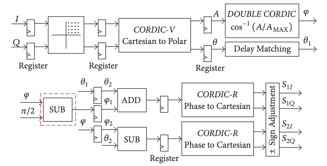
SCS 原理图如上图所示。其中基带 I Q 信号为 64QAM 信号。为了简化算法实现的复杂度,首先将 I Q 信号变换到第一象限,并记录下 I Q 信号原本的象限,最后在输出的时候做符号调整就可以了。上图红框中将 \(\varphi - \pi/2\),原因是因为在实际的设计过程中发现 \(\theta + \varphi\) 会大于 \(\pi /2\),为了避免溢出而将其减了 \(\pi /2\),因此在进行符号调整之前: \[ S_{1I}(t) = 0.5 A_{max} \rm{cos}[\theta(t)+\phi(t) - \pi/2] \]

\[ S_{1Q}(t) = 0.5 A_{max} \rm{sin}[\theta(t)+\phi(t)-\pi/2] \]

Matlab 行为级仿真

在进行 MATLAB 仿真时,为了让仿真结果和真实结果更加接近,进行了每一步计算过程都进行了浮点转定点数的操作。

仿真结果

  1. 64QAM 基带信号:

    64QAM基带信号
  2. 64QAM 频带信号:

    QAM信号波形
  3. 64QAM 星座图:

    QAM信号星座图
  4. 对基带信号进行 SCS 运算得到的 \(S_{1I},S_{1Q},S_{2I},S_{2Q}\) 信号:

    QAM基带信号信号SCS
  5. 将 SCS 后的基带信号与载波相乘:

    QAM信号SCS

    可以看到两路信号 S1 和 S2 是两路恒包络的调相信号,说明 SCS 模块实现了将原来的调幅调相信号转为两路恒包络的调相信号。

  6. 两路信号 S1 和 S2 合成:

    QAM信号SCS合成

    可以看到合成后的信号与原始信号一致,说明在 SCS 的过程中信号的信息没有丢失。

Matlab 代码

1
2
3
4
5
6
7
8
9
10
11
12
13
14
15
16
17
18
19
20
21
22
23
24
25
26
27
28
29
30
31
32
33
34
35
36
37
38
39
40
41
42
43
44
45
46
47
48
49
50
51
52
53
54
55
56
57
58
59
60
61
62
63
64
65
66
67
68
69
70
71
72
73
74
75
76
77
78
79
80
81
82
83
84
85
86
87
88
89
90
91
92
93
94
95
96
97
98
99
100
101
102
103
104
105
106
107
108
109
110
111
112
113
114
115
116
117
118
119
120
121
122
123
124
125
126
127
128
129
% main.m
clc
clear all
mkdir image

% fixed word length and fraction length bits
wl = 16;
fl_1 = 15;
fl_pi = 14;

M=64;
xmax = 8;
ymax = 8;
Amax = sqrt(xmax^2 + ymax^2);

msg = 0:1:63; %消息信号
% msg = random_msg([0 M-1], M);

ts = 0.01; %抽样时间间隔
T = 1; %符号周期
t = 0:ts:T; %符号持续时间向量
x = 0:ts:length(msg); %所有符号的传输时间
fc = 1; %载波频率
c = sqrt(2/T)*exp(1j*2*pi*fc*t); %载波信号
msg_qam = qammod(msg,M).'; %基带8-QAM调制
tx_i_qam = real(msg_qam*c); %载波调制
tx_q_qam = imag(msg_qam*c); %载波调制
tx_i_qam= reshape(tx_i_qam.',1,length(msg)*length(t));
tx_q_qam= reshape(tx_q_qam.',1,length(msg)*length(t));
% plot(x,tx_i_qam(1:length(x)),x,tx_q_qam(1:length(x)));
figure(1);
plot(x,tx_i_qam(1:length(x)));
title([num2str(M) 'QAM信号波形'])
xlabel("时间t");ylabel("载波振幅");
saveas(gcf, 'image/QAM信号波形.svg');
figure(2);
plot(1:length(msg_qam),real(msg_qam),1:length(msg_qam),imag(msg_qam))
legend('I','Q')
xlabel("时间t");ylabel("基带振幅");
tit = [num2str(M) 'QAM基带信号'];
title(tit);
saveas(gcf, ['image/' tit], 'svg');
% figure(2);
% scatterplot(msg_qam)
% title([num2str(M) 'QAM信号星座图'])
% xlabel("同相分量");ylabel("正交分量");

% CORDIC-V Cartesian to Polar
% 将 QAM 信号变换到第一象限,并记录下符号
[msg_qam_tarns, msg_qam_symbol] = transform(msg_qam);
x_qam = real(msg_qam_tarns);
y_qam = imag(msg_qam_tarns);
% Construct signed fixed-point numeric object
% 将 x y 归一化到 [0, 1]
x_fixed = sfi(x_qam/xmax, wl, fl_1);
y_fixed = sfi(y_qam/ymax, wl, fl_1);
% Theta (0, pi/2), r (0, sqrt(2))
[Theta,r] = cordiccart2pol(x_fixed, y_fixed);
% % 将 r 归一化到 (0, 1)
r_fixed = sfi(r/sqrt(2), wl, fl_1);
Theta_fixed = sfi(Theta, wl, fl_pi); % fixed

% DOUBLE CORDIC
% r_fixed (0, 1), Varphi [0, pi/2]
Varphi = cordicacos(r_fixed);
Varphi_fixed = sfi(Varphi, wl, fl_pi); % fixed

% CORDIC-R Phase to Cartesian
Phase_S1 = Theta_fixed + Varphi_fixed - pi/2; % 将 Phase_S1 限制在 (-pi/2, pi/2)
Phase_S2 = Theta_fixed - Varphi_fixed; % Phase_S2 在 (-pi/2, pi/2)
Phase_S1_fixed = sfi(Phase_S1, wl, fl_pi);
Phase_S2_fixed = sfi(Phase_S2, wl, fl_pi);

S1_I_tmp = 0.5*Amax*cordiccos(Phase_S1_fixed);
S1_Q_tmp = 0.5*Amax*cordicsin(Phase_S1_fixed);
S2_I_tmp = 0.5*Amax*cordiccos(Phase_S2_fixed);
S2_Q_tmp = 0.5*Amax*cordicsin(Phase_S2_fixed);

# Signal Adjusment
[S1_I, S1_Q, S2_I ,S2_Q] = Signal_Adjusment_quad(S1_I_tmp, S1_Q_tmp, S2_I_tmp, S2_Q_tmp, msg_qam_symbol);

tt = 1:1:64;
figure(3);
tiledlayout(2,1)
ax1 = nexttile;
plot(ax1, tt,S1_I, tt,S1_Q);
legend(ax1, 'S_{1I}', 'S_{1Q}')
title(ax1, "QAM基带信号信号SCS S1")
xlabel(ax1, "时间t");ylabel(ax1, "振幅");
ax2 = nexttile;
plot(ax2, tt,S2_I, tt,S2_Q);
legend(ax2, 'S_{2I}', 'S_{2Q}')
title(ax2, "QAM基带信号信号SCS S2")
xlabel(ax2, "时间t");ylabel(ax2, "振幅");
saveas(gcf, 'image/QAM基带信号信号SCS', 'svg');

% 调制
S1 = real(((S1_I+1j*S1_Q)')*c); %载波调制
S2 = real(((S2_I+1j*S2_Q)')*c); %载波调制
S1= reshape(S1.',1,length(S1_I)*length(t));
S2= reshape(S2.',1,length(S2_I)*length(t));
figure(4);
tiledlayout(2,1)
ax1 = nexttile;
plot(ax1, x,S1(1:length(x)))
legend(ax1, 'S1')
title(ax1, [num2str(M) 'QAM信号SCS S1']);
xlabel(ax1, "时间t");ylabel(ax1, "振幅");
ax2 = nexttile;
plot(ax2, x,S2(1:length(x)))
legend(ax2, 'S2')
title(ax2, [num2str(M) 'QAM信号SCS S2']);
xlabel(ax2, "时间t");ylabel(ax2, "振幅");
saveas(gcf, 'image/QAM信号SCS', 'svg');

S = S1 + S2;
figure(5);
plot(x,S(1:length(x)));
legend('S')
title([num2str(M) 'QAM信号SCS合成']);
xlabel("时间t");ylabel("振幅");
saveas(gcf, 'image/QAM信号SCS合成', 'svg');

% 星座图
% figure(6)
scatterplot(msg_qam);
title([num2str(M) 'QAM信号星座图']);
xlabel("同相分量");ylabel("正交分量");
saveas(gcf, 'image/QAM信号星座图', 'svg');
1
2
3
4
5
6
7
8
9
10
11
12
% random_msg.m
% 生成随机序列
%
function msg = random_msg(range, lenght)
% 首先,初始化随机数生成器,以使本示例中的结果具备可重复性。
rng(0,'twister');
% 创建一个 M 个随机值的向量。使用 rand 函数从开区间 (0,M-1) 抽取均匀分布的值。
a = range(1);
b = range(2);
r = (b-a).*rand(1,lenght) + a;
msg = round(r);
end
1
2
3
4
5
6
7
8
9
10
11
12
13
14
15
16
17
18
19
20
21
22
23
24
25
26
27
28
29
30
31
32
33
34
35
% Signal_Adjusment_quad.m
function [S1_I, S1_Q, S2_I ,S2_Q] = Signal_Adjusment_quad(S1_I_tmp, S1_Q_tmp, S2_I_tmp, S2_Q_tmp, symbol)
len = length(S1_I_tmp);
S1_I = zeros(1, len);
S1_Q = zeros(1, len);
S2_I = zeros(1, len);
S2_Q = zeros(1, len);
for i = 1:1:len
if symbol(i,:) == [1, 1]
% 第一象限
S1_I(i) = -S1_Q_tmp(i);
S1_Q(i) = S1_I_tmp(i);
S2_I(i) = S2_I_tmp(i);
S2_Q(i) = S2_Q_tmp(i);
elseif symbol(i,:) == [-1, 1]
% 第二象限
S1_I(i) = -S2_I_tmp(i);
S1_Q(i) = S2_Q_tmp(i);
S2_I(i) = S1_Q_tmp(i);
S2_Q(i) = S1_I_tmp(i);
elseif symbol(i,:) == [-1, -1]
% 第三象限
S1_I(i) = S1_Q_tmp(i);
S1_Q(i) = -S1_I_tmp(i);
S2_I(i) = -S2_I_tmp(i);
S2_Q(i) = -S2_Q_tmp(i);
else
% 第四象限
S1_I(i) = S2_I_tmp(i);
S1_Q(i) = -S2_Q_tmp(i);
S2_I(i) = -S1_Q_tmp(i);
S2_Q(i) = -S1_I_tmp(i);
end
end
end

Reference

[1] CORDIC-Based Multi-Gb:s Digital Outphasing Modulator for Highly Efficient Millimeter-Wave Transmitters

[2] A Sub-mW All-Digital Signal Component Separator With Branch Mismatch Compensation for OFDM LINC Transmitters

[3] A Low Power All-Digital Signal Component Separator for Uneven Multi-Level LINC Systems

-------The end of this article  Thank you for your reading-------